Risk management - Simple estimating of risk
Simple estimating of risk
This is a process you could use as part of the Evaluation phase.
Let us say that if a particular risk occurs you have to estimate a possible delay to the project.
You may consider a range of possibilities in terms of:
| MAXIMUM: | 11 weeks |
| LIKELY: | 9 weeks (in between and considered the most probable) |
| MINIMUM: | 7 weeks |
You can’t be sure that these accurate values as indicated will be correct as there will be a degree of doubt based upon available data and experience.
In this case, you need to apply a range for each of these. It seems logical that as the MAXIMUM and MINIMUM values are equidistant from the LIKELY value the range should be + and – half the difference. This would give a range of + or – 1 week, and thus ranges of:
| MAXIMUM: | 10 to 12 weeks |
| LIKELY: | 8 to 10 weeks |
| MINIMUM: | 6 to 8 weeks |
You need to have some idea how likely each of these ranges are to occur.
You could consider the following likelihoods:
| MINIMUM: | 20% or 0.2 chance of occurrence |
| MAXIMUM: | 30% or 0.3 chance of occurrence (slightly increased chance) |
| LIKELY: | 50% or 0.5 (i.e. 100% or 1.0 minus the sum of the others and the most likely) |
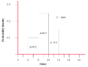
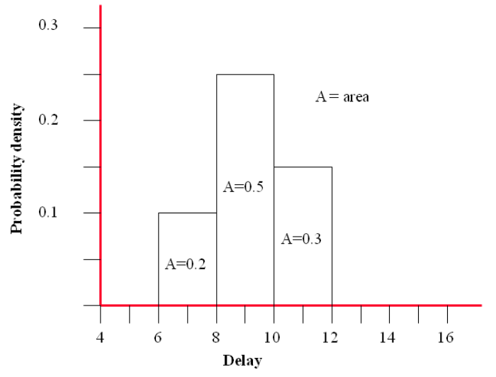
If you then plot a graph of the ‘delay’ ranges where the area of each column is equal to the ‘likelihood’ you will have a ‘Y-axis’ that equates to the Probability density.
That is:
Area under the column = probability density x delay range
Or for the MINIMUM range
Area = 0.1 x 2 = 0.2 (i.e. 20 % probability of occurrence)
The graph represents the PROBABILITY DENSITY FUNCTION (PDF).
You now need to assess the LIKELIHOOD of the risk occurring at all.
Let us say you believe there to be a 30% chance of occurrence. In other words, simplistically, if you were able to run exactly the same project 10 times the risk would materialise on 3 occasions and not appear on 7 of them.
The Probability Density Function allows us to derive a truer idea of the actual delay by looking at the likelihood of the individual ranges.
You can see from the graph that there is a slightly higher probability that the actual delay will be higher than 9 weeks and not less.
A simple calculation would show the contributions from each range:
MINIMUM = probability x minimum value = 0.2 x 7 = 1.4 weeks contribution
LIKELY = probability x likely value = 0.5 x 9 = 4.5 weeks contribution
MAXIMUM = probability x maximum value = 0.3 x 11 = 3.3 weeks contribution
The overall contribution to the delay is:
1.4 + 4.5 + 3.3 = 9.2 weeks.
If each man week cost £1000 the overall cost of delay could be 9.2 x £1000 = £9,200
However, we have said that the chances of the risk materialising is only 30%.
So, the appropriate cost to add to the budget would be £9,200 x 30% = £2760.
If the likelihood of the risk occurring had been 20% the cost for the budget will be £9,200 x 20% = £1,840
So why don’t we just add £9,200 to the budget?
It is because you are not managing one risk but many, some of which will not occur.
For example, in simple terms, if we had 10 risks and each was given a 20% chance of occurrence they would not all occur (unless you were very unlucky).
Out of 10 you would expect 2 of them to occur but you could not predict which two. If we said the cost of each risk occurring is £2000 then the overall cost would be £20,000 if they all occurred.
We will only allow for 20% of each in the budget which is £400 x 10 = £4000. If, statistically, only 2 occur the cost will be £2000 x 2 = £4000!
So, the budget should cover it. This is why it is necessary to estimate well because if you don’t many more risks will surface than you have allowed for destroying your budget.
We can look at the estimate in a slightly different way.
We have already said that the likelihood of the risk materialising is 20% therefore the likelihood of the risk not occurring is 80%. So, there is an 80% chance of the impact being 0 weeks.
We can represent this as:
| Impact (weeks) | Probability |
| 0 | 0.8 |
| 7 | 0.2 x 0.2 = 0.04 |
| 9 | 0.5 x 0.2 = 0.10 |
| 1 | 0.3 x 0.2 = 0.06 |
Note: the total probability of the others occurring must add up to 0.2.
The probability of each one will be:
The probability estimate x 0.2 (the 1.0 – 0.8).
If we now use the probabilities above to work out the impact we have:
7 x 0.04 = 0.28
9 x 0.10 = 0.90
11 x 0.06 = 0.66
Giving a total = 1.84 weeks (conditional)
We saw previously that if we just look at the original probabilities of 0.2, 0.5 and 0.3 for the ranges we found:
7 x 0.2 = 1.4
9 x 0.5 = 4.5
11 x 0.3 = 3.3
Giving a total = 9.2 weeks (unconditional)
The first is based upon the ‘condition’ that the risk has a 20% chance of occurring.
The second ignores this and is ‘unconditional’.
So, the value of 1.84 weeks represents the cost value on the basis that the risk only has a 20% chance of materialising based also upon a range of values.
That is:
Unconditional value x probability of the risk occurring = conditional value
9.2 X 0.2 = 1.84 weeks.
If the cost is £2000 per week the budget would include 1.84 x £2000 = £3,680.
If the cost is £1000 per week the budget would include 1.84 x £1000 = £1,840. (check with the example above)
The process of estimating the likelihood of range values can be taken one or two steps further.
[see Simple estimating of risk more detail].
We can convert the information in the above diagram to a Cumulative probability graph [see Cumulative probability graph].