Risk management - Monte Carlo risk distribution
Monte Carlo risk distribution
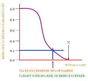
Whilst the previous histogram [see Monte Carlo simulation output] has its uses it isn’t very easy to view risk. Project managers will find it easier to view the data in the histogram in another format.
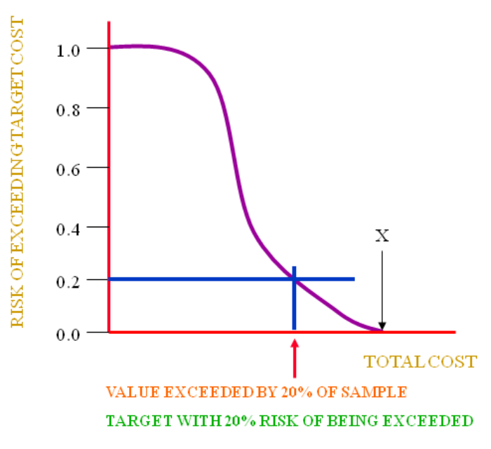
The risk distribution graph above does that.
In the above graph the 2 axes are:
‘x’ axis
Total cost as before [see Monte Carlo simulation output].
‘y’ axis
The other is the ‘risk of exceeding the target total’
Basically, all values must be higher than zero (that is 100% or 1.0).
Similarly, the ‘total cost’ can not exceed ‘X’ or in this case £200,000, so, the probability is 0% or 0.0 in the above graph.
All other ‘total cost’ values will lie somewhere in between but the relationship is not linear.
In fact, there is little change in the probability for the occurrence of ‘total cost’ at the lower end. The risk then begins to drop more rapidly in the middle values and slows down at the upper end.
Another way of looking at the middle values is that they are more common, they are more likely to arise. We can see from the previous histogram [see Monte Carlo simulation output] that the majority of ‘total cost’ values lie somewhere in the middle. This is what we might expect.
However, the problem with this region, is that the RISK is more sensitive. For a small change in the ‘total cost’ the risk can change a lot.
What we have to remember is the point of the ‘total cost’ in the project.
When you propose a ‘total cost’ you are doing this for a reason, to set a budget or to provide a quote to obtain a contract.
Naturally, you would like to set a ‘total cost’, (the same would apply to durations and the final completion date), that is low enough to get the contract. If however, you set it too low, for example near the middle, then there will be a very good chance that you won’t achieve it as the RISK sensitivity is too high.
If on the other hand, you if set it too high, it may be a much lower risk, but you could lose the contract.
From realistic example we could have a MINMUM cost of £50,000 and a MAXIMUM cost of £250,000. The actual cost of the project will lie somewhere within this range.
If you set the final project cost at about half way (£150,000, i.e. midway between £50,000 + £200,000) there is a (approximately) a 60% risk of it being exceeded. So there is a high risk that there will be a negative impact on the project.
So, you may get the contract, but at what cost, as the quoted ‘total cost’ has a very good chance of being exceeded.
So where do we set the ‘total cost’.
In order to manage a low risk (in a less sensitive region of the graph) it is better to set the ‘total cost’ at a 20% risk of being exceeded.
If the individual activity ranges were realistic then this allows a reasonable margin to reduce the quote without altering the risk so drastically that it will be exceeded.
This indicates why it is so important in the ‘estimate’ phase of the risk management process to do a good job.
So, in our case we could quote a ‘total cost’ for the project of say£210,000 (assuming this is the ‘total cost’ that 800 simulations do not exceed).
This would therefore be competitive for the contract and at the same time have a lower risk of being exceeded.