Risk management - Task probability
Task probability
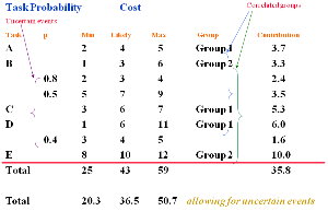
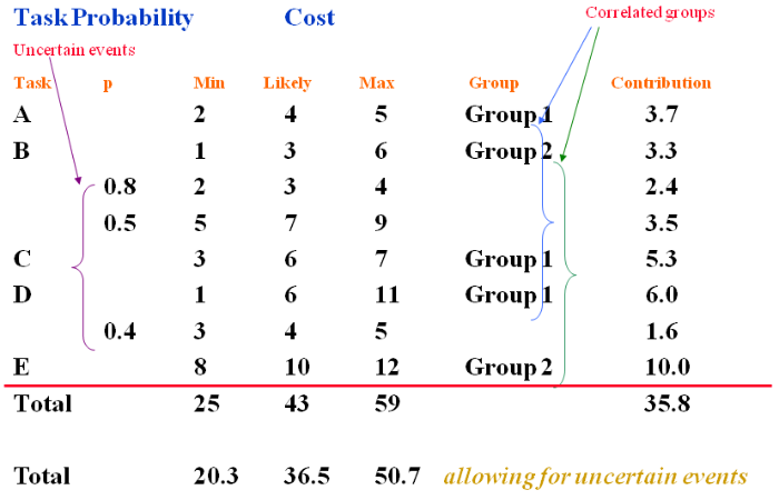
The above diagram shows us how risk management software may use the data to generate a random number of samples.
Let us first look at the column headings.Task
(or Work Package. This could be a group of tasks summarised in a high level plan)
For simplicity we will use 5 i.e. A, B, C, D and E.
Note: That in this case task B has 2 uncertain events (risks) and task D one uncertain event associated with it. The plan will contain ‘proactive’ responses to these risks.
PThis is the probability that the uncertain events (risks) may occur.
For example, for the first uncertain event with Task B we have a probability that it will occur of 0.8. This can also be given as 80%.
Therefore, there is 20% chance that it will not, or 0.2. The second risk is judged to have 50% likelihood of occurrence.
Note: These values do not add up to 1.0 (i.e. 0.8 + 0.5). We are assessing the likelihood of separate events occurring, each of which may or may not materialise.
Also, the probabilities are only less than 1.0 for the uncertain events. This is because the probability for the other Tasks (A, B, C, D, and E) to occur will be 1.0 as these will occur and are planned for.
Min, Likely and Max.
As we have seen before [see Simple estimating of risk] these are the 3 point estimates for each of the tasks and for the uncertain events.
Note: The ‘3 point estimate’ acts as a constraint. When the computer software assigns random values to simulate the events they can not lie outside the MINIMUM and the MAXIMUM values.
GroupIf you remember we said earlier that there may well be a ‘correlation’ between particular tasks.
Those tasks that have a common underlying driver, so that they are ‘correlated’ are put into like groups.
These can be called anything that you wish and may represent the type of correlation to which they refer.
In the above case, Tasks A, C and D are correlated as Group 1.
Tasks B and E are correlated as Group 2.
Drivers could be:
- The resource is identical for both tasks e.g. contractors or general labour.
- The same equipment is being used in both tasks.
- Estimation of the times involved for each task was based upon similar assumptions or persons generating the information.
One member of a correlated group has to be designated as independent. In a spreadsheet this is usually the first one in the row.
The value assigned to the independent task then drives all the others correlated to it using a particular factor.
This is a method of weighting the impact of the 3 point estimate of each task.
If we look at task ‘A’ we have a 3 point estimation of:
| MINIMUM | = 2 |
| LIKELY | = 4 |
| MAXIMUM | = 5 |
If we add these values together we get = 11
If we divide this by 3 we get = 3.7
This seems sensible as it reflects the most likely value. If the most likely value had been 2.5 then the contribution would have been:
(2 + 2.5 + 5 ) divided by 3 = 3.2, a lower weighting.
For a RISK ASSESSMENT we need to go through many cycles (simulations) in order generate a range of total costs along with their frequency of occurring.
For each cycle a random value of the cost is chosen for each Task and then summarised to give a total project cost.
Where an uncertain event occurs we need to allow for its probability of occurring.
For example, in task ‘B’ above we have an uncertain event with a probability of occurring of 0.8 (80%).
We are saying that it will occur on average 8 times in every 10 iterations. So, the software takes this into account and only allows it to make a contribution at intervals as in the real world.
The contribution value for an uncertain event is:
Sum of 3 point estimates e.g. 2 + 3 + 4 = 9,
Divided by 3 = 3
Then multiplied by its probability of occurrence, i.e. x 0.8 = 2.4.
If we took a simplistic view and just added up all of the MINIMA, LIKELY and MAXIMA scores for each task we would end up with the total:
Allowing for the actual probability of the uncertain events.
| MINIMUM | = 20.3 |
| LIKELY | = 36.5 |
| MAXIMA | = 50.7 |
Had we not allowed for their probabilities and assumed they were 100% it would have been:
| MINIMUM | = 25 |
| LIKELY | = 43 |
| MAXIMA | = 59 |
Significantly different.
So, all of the most LIKELY values, for each task, would give a total of 36.5.
However, the ‘contribution’ reflects the spread of the range (which differs for each task) and the relative position of the most likely value.
This total is 35.8, slightly less than the total of the likely values alone.
Note: The above diagram represents one iteration of the cycle for the most LIKELY values.
The summation of all the ‘contributions’ will represent the total cost for these ‘most LIKELY’ values which have been weighted.
In similar fashion, the software will choose random values for each of the tasks for each iteration (correlated groups will shadow the independent one).
Provided the iteration process is carried out somewhere between 300 to 1000 times we will generate enough ‘samples’ of the ‘total value’ to reflect real life.
This will give us a PDF of frequency (number of each total cost) versus total cost.
That is, we will have generated a range of ‘total costs’ from the absolute minimum (SUM of all the MINIMA) to the maximum (SUM of all the MAXIMA). The peak of the MONTE CARLO distribution will be somewhere in the middle.
This can then be converted to the more manageable graph of:
LIKELIHOOD (scale 0 to 1.0, chance of exceeding a particular ‘total cost’) versus TOTAL COST.
This is the graph that will allow us to see the RISK OF EXCEEDING a particular cost in terms of a PERCENTAGE.
In addition to finding the total cost of the project there is no reason why the simulations can not calculate sub totals at the same time. This will allow you to see more detail at various stage in the project.